This page contains examples of Veles visualization. For explanation on how they actually work check out Binary visualization explained.
By testing Veles visualizations on numerous files we found that different types of data look very differently.
We can easily notice the differences between a bitmap, a mobi file, a java .class file and an x86 compiled binary.

On a side note – visualizations of compressed or encrypted data look like a bunch of noise. Any trace of pattern in the visualized data immediately stands. For example, compare the gpg encrypted data and a .zip archive below. visualization makes it easy to spot headers in a zip archive. By switching to a “layered digram” mode of visualization we can immediately locate the headers at the end of the file. And not only that – we can also recognize certain patterns in the compressed stream (like the line on the right side of image).
Back to compiled binaries. We found out that any machine code looks roughly similar, but different architectures have their characteristic traits that can be used to recognize them. Below is the same binary compiled using three different architectures:
Ok, now let’s take a look at a specific file. For this demo, we’ll use libc.so from ubuntu 14.04.
|
1 2 |
> file libc-2.22.so libc-2.22.so: ELF 64-bit LSB shared object, x86-64, version 1 (GNU/Linux), dynamically linked (uses shared libs), for GNU/Linux 2.6.32, not stripped |
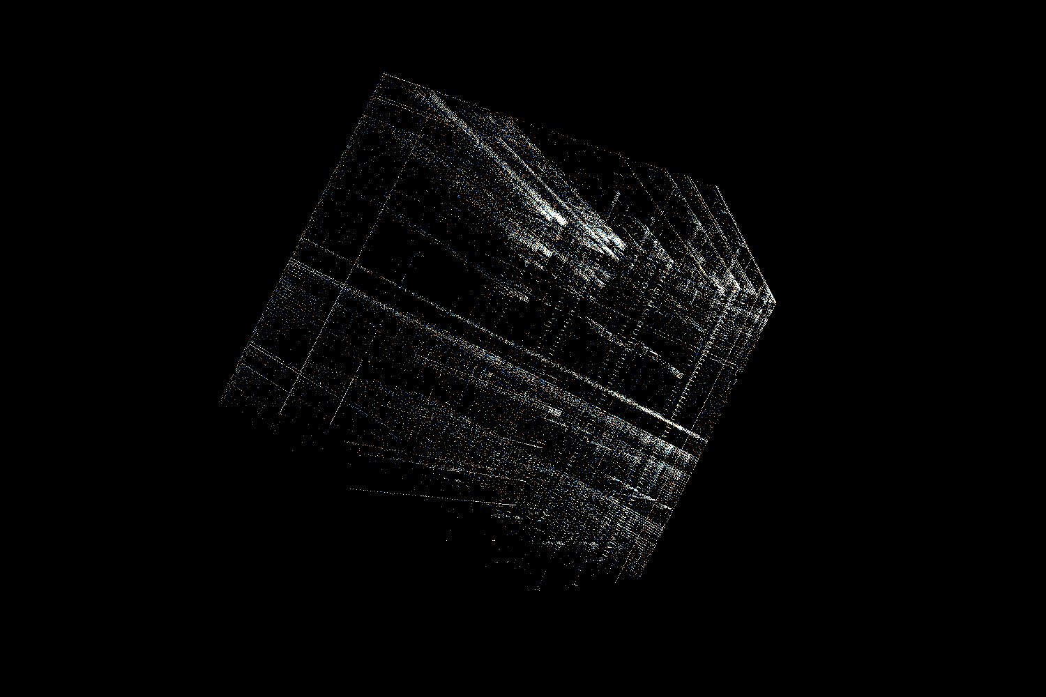
Recognising x86-64 architecture
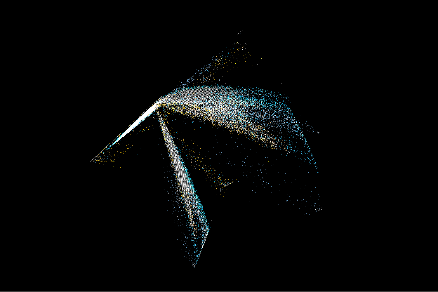
As mentioned in the video, we can recognise x86-64 code by finding 2 characteristic bars in the trigram view. Such a pair of bars means that there is a common sequence of 2 similar bytes (let’s call them x and y). One of the bars will correspond to trigrams <something, x, y>, while the second bar will be made of trigrams <x, y, something>.
So why do we see these bars in x86-64 machine code? It turns out that the default operand size for many instructions in 64-bit mode is 32 bits. If we want to use a 64-bit register we need to add a REX prefix. That means we prefix the instruction opcode with an additional byte with a value 0x40 + flags on lower 4 bits. In particular, many variants of MOV instruction will have a 2 byte opcode 0x4X 0x8Y (where X and Y depend on exactly which version of the instruction we used). Since MOV is an extremely common instruction, there will be a lot of those digrams in any x86 64-bit binary and we will clearly see the bars in trigram view. It’s also worth mentioning that another common instruction – LEA – happens to have 0x4X 0x8D opcode, which makes the bars even more visible.
.gnu.hash
As mentioned in the video the .gnu.hash section of ELF is made of 3 distinct parts:
-
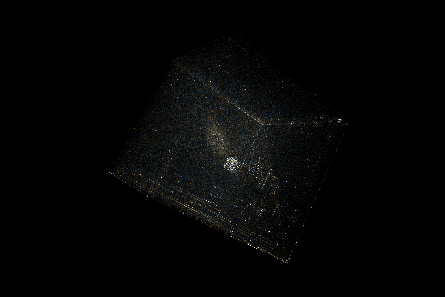
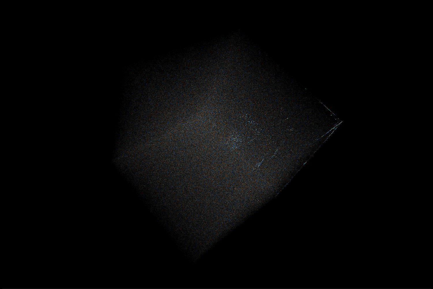
Bloom filter
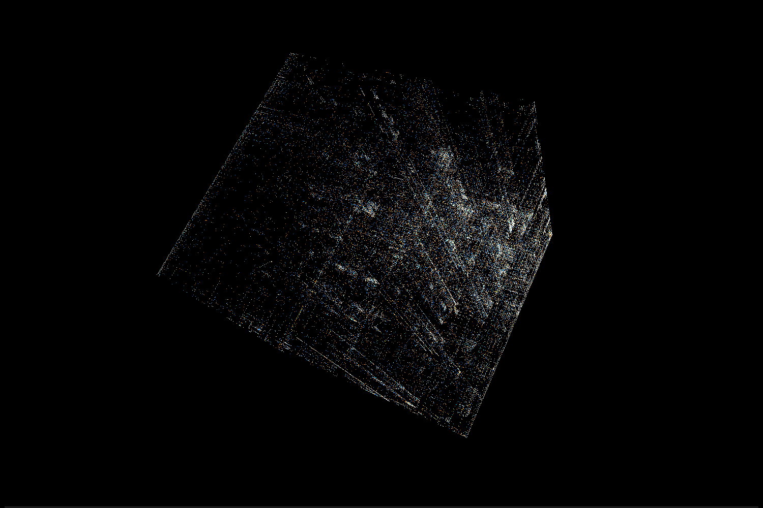
This is a probabilistic set with a possibility of false positives. Basically, when inserting an object it’s hashed into a few bit locations and all those bits are set to 1. To check if the object is already in the set we can just check all of those bits – if at least one of them has a value of 0 then we know the object is not in the set. The idea behind including this in the ELF is to avoid (if possible) the more expensive hashmap lookups.
In the visualization we can see that the Bloom filter is mostly random, but there are significantly more 0 bits than 1 bits in it. There are more numbers near the (0, 0, 0) corner of the cube. Additionally, we can see clusters of points near positions corresponding to values with just one or two 1s in binary representation.
-
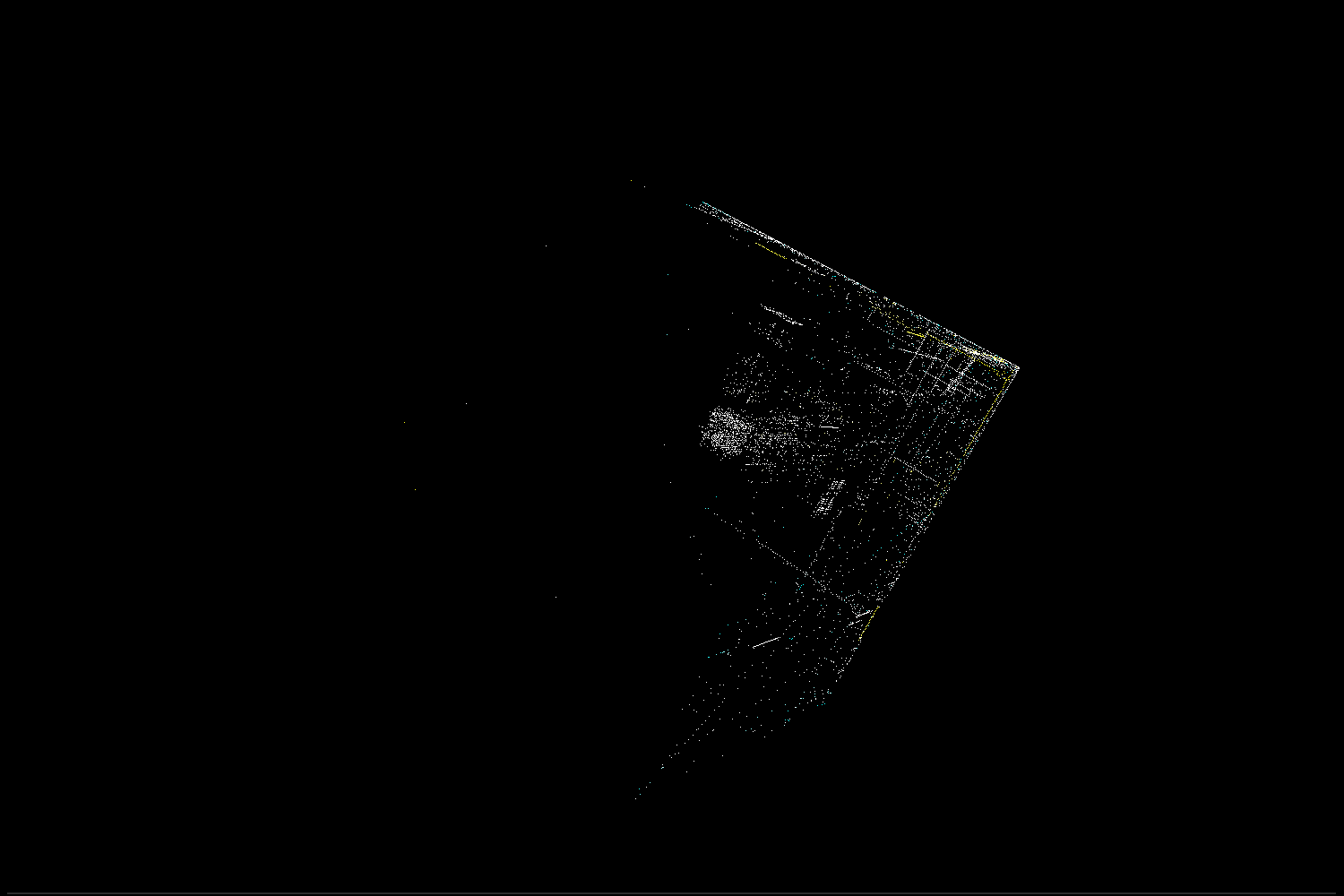
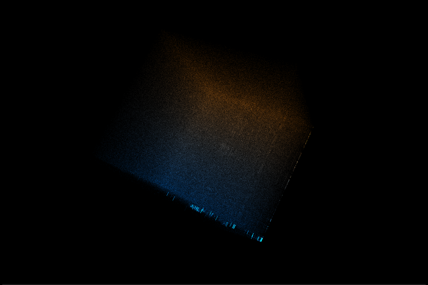
Hash buckets
Each value is the lowest index in the dynamic symbol table corresponding to a given hash. What we see in the visualization is relatively small values represented on 32-bit integers.
-
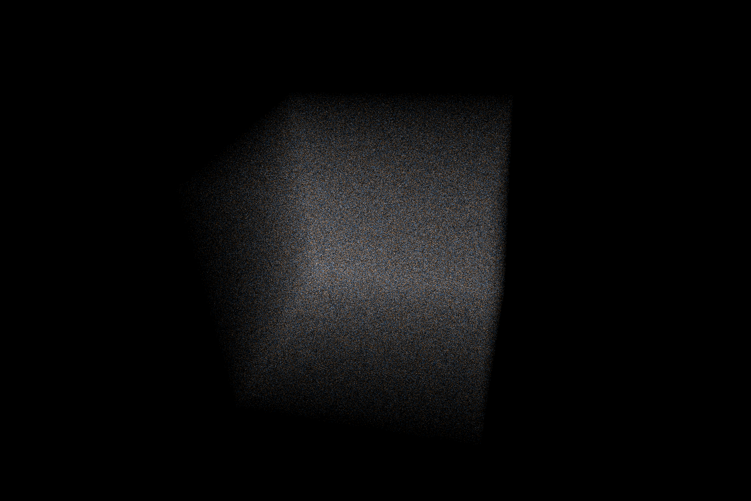
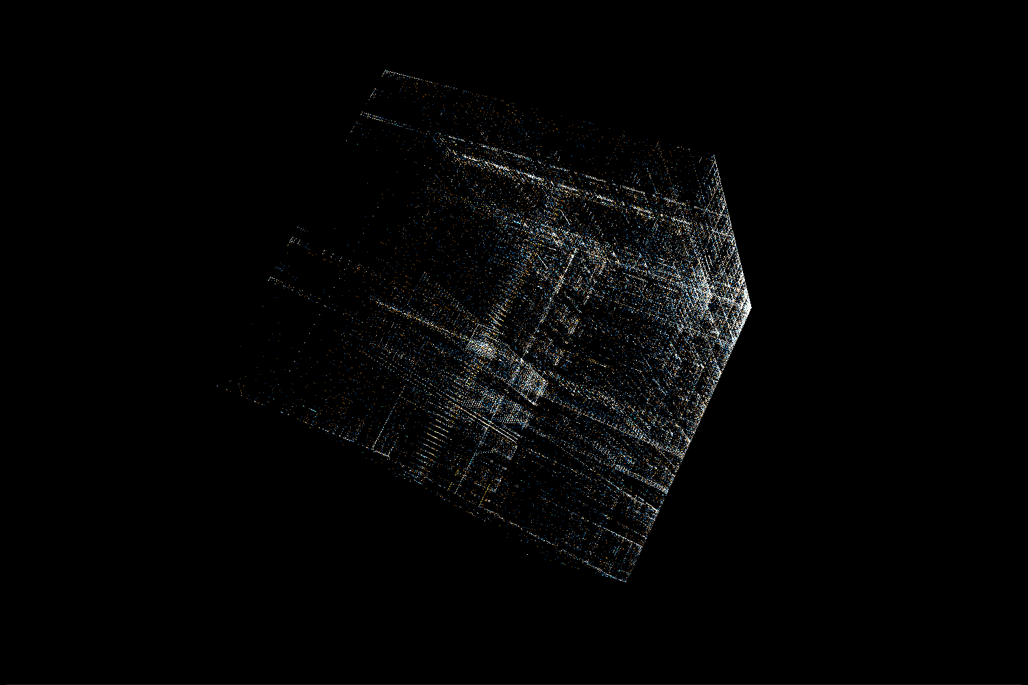
Hash values
These are computed hash values. As expected, they look like a bunch of white noise in a visualization.
For a more detailed description of how this section works, check out this link
[…] Binary data visualization 5 by dmit | 1 comments on Hacker News. […]